How do you mitigate the problem of class imbalance, and why is it important?
Class imbalance
- Occurs when one class has significantly fewer samples compared to others, especially in rare-event classification. E.g:
- Medical diagnosis
- Fraud detection
- Consequence: This can cause the model to be biased in favor of the majority class, resulting in poor predictive performance for the minority (which is often of greater interest)
- This may be disguised in the overall performance metrics.
-
Collect more data: While obvious, this should be your first thought!
-
Resampling
- Oversampling the minority class
- Under-sampling the majority class
- Both
-
Generate Synthetic Data: Use data augmentation techniques or synthetic data generation methods to create additional samples for the minority class. Note that this only applies to specific types of data.
-
Re-engineering the model
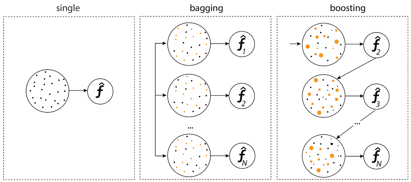
- Use ensemble methods such as bagging or boosting, which have better performance on imbalanced datasets. Bagging and boosting can help in reducing the variance caused by imbalances. Read here for the difference between bagging and boosting.
- Assign higher misclassification costs to the minority class in order to make the model more ‘careful’
- Anomaly Detection: Treat the problem as an anomaly detection task if the minority class is small enough to be treated like an anomaly.
The reason class imbalance is a problem is that most machine learning algorithms are designed to optimize overall accuracy, which can be misleading when one class dominates. They tend to predict the majority class for most instances, leading to poor predictive performance, especially for the minority class.
Question: Mitigating Class Imbalance in Machine Learning
How can one mitigate the problem of class imbalance in machine learning models, and why is addressing this issue crucial for model performance?
-
Importance of Addressing Class Imbalance:
- Class imbalance can lead to biased models that favor the majority class, resulting in poor predictive performance on the minority class, which is often of greater interest.
- In scenarios like fraud detection, medical diagnosis, or rare event prediction, the minority class is usually more significant despite its fewer instances.
-
Strategies for Mitigating Class Imbalance:
-
Resampling Techniques:
- Oversampling the Minority Class: Increase the number of instances in the minority class by duplicating them or generating synthetic samples (e.g., using SMOTE - Synthetic Minority Over-sampling Technique).
- Undersampling the Majority Class: Reduce the number of instances in the majority class to match the minority class size.
-
Algorithmic Ensemble Methods:
- Use ensemble techniques like Random Forests or Boosting algorithms that can be more robust against class imbalance.
- Implement boosting variants designed for imbalance, such as AdaBoost, which can focus more on hard-to-classify instances.
-
Cost-sensitive Learning:
- Adjust the algorithm’s cost function to penalize misclassifications of the minority class more than those of the majority class, making the model more sensitive to the minority class.
-
Threshold Moving:
- Adjust the decision threshold used by the classifier to change the trade-off between precision and recall, making the model more inclined to predict instances as the minority class.
-
↳ Follow-up Question:
Can you provide a real-world example where class imbalance might significantly impact model performance, and how would you apply the above strategies to mitigate this issue?
- Selection of Metrics: The choice of evaluation metrics should align with the specific nature of the problem. For example, in a highly imbalanced classification dataset, precision, recall, and the F1-score are more informative than accuracy.
↳ How can you actually measure a model’s performance on imbalanced datasets?
Better metrics for imbalanced datasets
In the presence of class imbalance, traditional metrics like accuracy can be misleading. Metrics such as Precision, Recall, F1-score, or the Area Under the Receiver Operating Characteristic Curve (AUC-ROC) provide a more nuanced view of model performance, especially for the minority class.
Evaluation metrics such as:
- Precision
- Recall
- F1-Score
- ROC-AUC
harder ones
-
Precisiona t.
-
Mean Average Precision (MAP): This is used to compute the average precision value for recall value over a certain threshold. It’s an extension of precision at k and is particularly useful in information retrieval.
-
Confusion Matrix: A confusion matrix is a table used to describe the performance of a classification model on a set of test data for which the true values are known. It includes true positives, false positives, true negatives, and false negatives, which are essential for understanding the model’s performance.
-
Mean Reciprocal Rank (MRR): MRR is a statistic measure for evaluating any process that produces a list of possible responses to a sample of queries, ordered by probability of correctness.
-
Normalized Discounted Cumulative Gain (NDCG): Used in information retrieval, NDCG measures the effectiveness of a model by looking at the ranking quality, taking into account the position of the correct labels.
-
Precision-Recall Curve: This is a plot that shows the trade-off between precision and recall for different thresholds. A high area under the curve represents both high recall and high precision.
Multi-class confusion matrix
Could you name some resampling methods?
- Simply duplicate existing samples
- Bootstrap sampling
Bootstrap Sampling
Read more about the math here
- SMOTE
SMOTE
Synthetic Minority Oversampling Technique
Given one bootstrap sample, what percentage of the original data is expected to be in the new dataset?
Around . To see the math behind this number, go here.
↳ Discuss the implications of this percentage for model validation, particularly in the context of variance and bias in the results obtained from bootstrap samples.
You mentioned bagging and boosting. What is the difference between the two methods?
Bagging is a method of merging the same type of predictions. Bagging decreases variance, not bias, and solves over-fitting issues in a model.
Boosting is a method of merging different types of predictions. Boosting decreases bias, not variance.
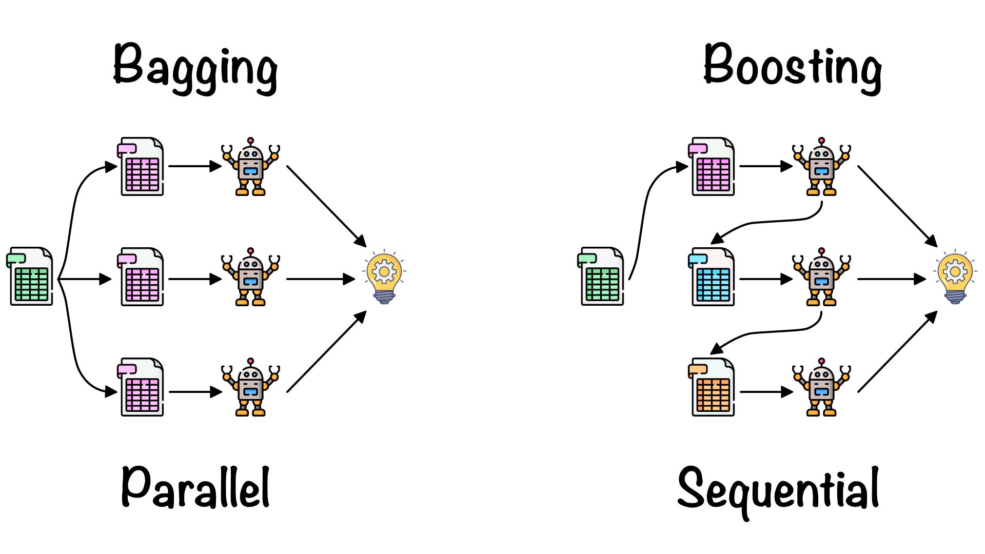
Note the independence Note the dependence
What is outlier detection?
Anomaly detection
Also known as outlier detection, is the process of identifying data points, events, or observations that deviate significantly from the dataset’s normal behavior. Three types: point, collective, and contextual anomalies
- Fraud
- Network intrusions
- Structural defects
- Health related issues
Question Here
Data enrichment. Kind of like data linking. Let’s say we have data on a list of company’s. We could enrich this dataset by combining it with a separate dataset with companies and their number of employees. We gain information for free, and thus can produce more powerful models.
What makes a model actually good?
What do you mean by ‘powerful model’.
It actually relates to the statistical definition ‘power’ (link) - the probability that the model is actually correct
Simp. Mew. go
How do we measure how good a model is?
Meaning of semantics.
How do you keep track of a model’s performance once it’s been deployed?
- Continuously track key performance indicators (KPIs) relevant to the model, the usual:
- accuracy
- precision
- recall
- F1 score
- ROC-AUC…
- For regression models, metrics like:
- Mean Squared Error (MSE)
- Root Mean Squared Error (RMSE)
- Mean Absolute Error (MAE)
- Monitor data drift
- Monitor concept drift
- Error analysis
Model Drift
There are two types:
- Concept Drift (the underlying relationship between x and y changes)
- Data Drift (the underlying distribution of the input changes)
Concept Drift (Model Drift)
Over time, the statistical properties of the target variable, which the model is predicting, can change. This phenomenon, known as model drift or concept drift, can occur due to evolving trends, changing market conditions, or alterations in customer behavior.
- Routine model retraining
Why might a machine learning model not perform as well as initially intended? Discuss potential factors that could lead to suboptimal performance.
-
Data Quality Issues:
- Incomplete or biased datasets
- Incorrect data labeling
- Presence of outliers or noise in the data
-
Model Complexity:
- Overfitting: The model is too complex, capturing noise instead of the underlying pattern. It overfit to the training data, and thus performed poorly on the unseen real world data.
- Underfitting: The model is too simple to capture the underlying structure of the data.
-
Feature Engineering:
- Inadequate feature selection, leading to missing key predictors.
- Poor feature preprocessing and normalization.
-
Hyperparameter Tuning:
- Inappropriate hyperparameter values that do not suit the data or the problem.
-
Algorithm Selection:
- Choosing an algorithm that is not well-suited to the specific type of problem or data structure.
-
Evaluation Metrics:
- Relying on inappropriate or misleading performance metrics.
-
External Factors:
- Changes in the underlying data distribution over time (concept drift).
- Constraints on computational resources limiting model complexity or training time.
Callout Box: Understanding Model Generalization Generalization refers to a model’s ability to perform well on new, unseen data. A key goal in machine learning is to develop models that generalize well, rather than models that perform only exceptionally well on training data but poorly on new data.
How can one assess if a model is overfitting or underfitting, and what are the common strategies to address these issues?
Assessing Overfitting and Underfitting:
-
Performance Metrics: Evaluate the model’s performance on both the training and validation datasets. A significant gap between training accuracy and validation accuracy indicates overfitting, whereas poor performance on both may suggest underfitting.
-
Learning Curves: Plot learning curves by graphing the model’s performance on the training and validation sets over time (or over the number of training instances). Overfitting is indicated by a large gap between the training and validation curves, while underfitting is suggested by both curves plateauing at a low level of performance.
-
Cross-validation: Use cross-validation techniques to assess how the model’s performance generalizes across different subsets of the data. High variance in performance across folds may indicate overfitting.
Strategies to Address Overfitting:
-
Simplifying the Model: Reduce the complexity of the model by selecting a simpler algorithm or reducing the number of features or parameters.
-
Regularization: Apply techniques such as L1 or L2 regularization, which add a penalty on larger weights to prevent the model from fitting the training data too closely.
-
Pruning: In decision trees or neural networks, remove parts of the model (such as branches or neurons) that contribute little to the model’s predictive power.
-
Adding More Data: Increasing the size of the training dataset can help the model learn more generalized patterns.
-
Early Stopping: Monitor the model’s performance on a validation set and stop training when performance begins to degrade, preventing overfitting.
-
Dropout: For neural networks, randomly dropping units (along with their connections) during training can prevent co-adaptation of features and reduce overfitting.
Strategies to Address Underfitting:
-
Increasing Model Complexity: Move to a more complex model that can capture the underlying patterns in the data more effectively.
-
Feature Engineering: Create new features or transform existing ones to provide the model with more information about the underlying structure of the data.
-
Reducing Regularization: If regularization is too strong, it might prevent the model from fully learning the underlying pattern. Reducing regularization can help.
-
Longer Training Time: Ensure that the model has been trained for a sufficient number of epochs, allowing it to converge properly.
Callout Box: The Balance Act The key to successful machine learning models lies in balancing complexity and generalization. It’s crucial to find a sweet spot where the model is complex enough to capture the essential patterns in the data without being so complex that it starts to memorize the training data.
By carefully monitoring model performance and applying appropriate strategies, one can mitigate the issues of overfitting and underfitting, leading to more robust and effective machine learning models.
How do you predict customer revenue?
How can you predict churn? (at different time windows is useful)
We’ve seen a spike in churn rate, how can you figure out why? (think feature importance)
Deprecated but my Jupyter notebook question was about finding out what characteristics of people are important when determining how good a customer they are (also feature importance)
How can you deal with a categorical FEATURE in a model that only takes numerical inputs? (think one hot encoding, sequential encoding but only if it is appropriate/ordinal variable)
What do you do if you have a LOT of cardinality in the feature? (one hot encoding is a bad idea for something like postcodes, can you group them into states/LGAs/countries etc. instead so they’re still useful and not like 10,000 extra binary features)
You’re right to question the use of squaring the modulus. In the expression (| \epsilon - \hat{\epsilon} |^2), the notation (|\cdot|) usually refers to a norm, often the Euclidean norm in the context of vectors, which itself represents a kind of “distance” or “magnitude.” Squaring this norm is a common practice in various fields, including statistics and machine learning, for several reasons:
-
Emphasizing Larger Errors: Squaring magnifies larger differences more than smaller ones. This can be useful when the aim is to give more weight to larger errors.
-
Analytical Convenience: Squaring the norm often leads to mathematical expressions that are easier to differentiate and work with, especially in optimization problems.
-
Removing Sign: The square ensures that the result is always non-negative, regardless of the sign of (\epsilon - \hat{\epsilon}). This is useful when only the magnitude of the error matters, not its direction.
-
Euclidean Distance: When (\epsilon) and (\hat{\epsilon}) are vectors, (| \epsilon - \hat{\epsilon} |) represents the Euclidean distance between them, and squaring this norm gives the square of the Euclidean distance, which is a common measure in various algorithms.
So, the expression (| \epsilon - \hat{\epsilon} |^2) is indeed meaningful and correct depending on the context in which it is used. It represents the square of the norm (or distance) between (\epsilon) and (\hat{\epsilon}).
What is the “quality versus inference budget” tradeoff in ML?
Quality vs. Budget Tradeoff
The “quality versus inference budget tradeoff” is a concept often encountered in the field of machine learning, particularly in the context of deploying models in real-world applications. This tradeoff revolves around balancing the quality of the model’s predictions (accuracy, precision, reliability, etc.) with the resources required to generate these predictions (time, computational power, cost, etc.). Here’s a more detailed explanation:
What is the “bias versus variance” tradeoff in ML?
Here’s a few definitions to chew on.
Bias vs. Variance Tradeoff
The tradeoff between fitting the training data well and performing well on real/testing data.
Bias vs. Variance Tradeoff
In statistics and machine learning, the bias–variance tradeoff describes the relationship between a model’s complexity, the accuracy of its predictions, and how well it can make predictions on previously unseen data that were not used to train the model.
It’s essentially saying; you can learn all the patterns in the data, but at some point you’ll be learning random noise (unhelpful) specific to this particular training data, instead of useful signal that will be present in any real data.
The job of every single machine learning model is to learn patterns in the data. You want a sufficiently sophisticated model that it can learn these tiny clever little patterns in the data but eventually you can go too far and into learning just pure noise, the model thinks its being all cleer and whatnot but
An optimized model will be sensitive to the patterns in our data, but at the same time will be able to generalize to new data.
False/True Positive/Negative
The concept of signal will change the way you see the world
What things do we need to measure the ‘distance’ between in Machine Learning
In machine learning, measuring distances between different types of data is crucial for various algorithms and models. Here are some conceptual things where distance measurement is important, along with examples of machine learning models where these measures play a significant role:
-
Text Data:
- Models:
- Natural Language Processing (NLP) Models: These include models like BERT, GPT, and Transformer-based architectures where text embeddings are compared using distance metrics to understand semantic similarity.
- Text Classification Models: Such as Naive Bayes or Support Vector Machines (SVMs) that may use distance measures in feature space for classification tasks.
- Models:
-
Feature Vectors in General:
- Models:
- K-Nearest Neighbors (KNN): A distance-based classifier where the class of a sample is determined by the classes of its nearest neighbors in the feature space.
- Clustering Algorithms: Like K-means or Hierarchical clustering, where distance measures are used to group similar data points.
- Models:
-
Images:
- Models:
- Convolutional Neural Networks (CNNs): Used in image recognition and classification tasks. Distance measures can be used in the feature space after convolutional layers.
- Image Retrieval Systems: Where distances between image features are calculated for finding similar images.
- Models:
-
Time Series Data:
- Models:
- Dynamic Time Warping (DTW): Used in time series analysis, especially for speech recognition, where it measures the distance between two temporal sequences which may vary in speed.
- Recurrent Neural Networks (RNNs) and Long Short-Term Memory Networks (LSTMs): Used for analyzing time series data where distance metrics can be applied to the feature vectors in the hidden layers.
- Models:
-
Graph Data:
- Models:
- Graph Neural Networks (GNNs): Used in tasks like social network analysis, where distance measures can help in understanding the relationships and influence between nodes.
- Network Analysis Tools: Employed in analyzing and visualizing graph data, where distance metrics can be crucial for clustering and community detection.
- Models:
-
Multidimensional Data:
- Models:
- Principal Component Analysis (PCA): Used for dimensionality reduction, where distances in the high-dimensional space are preserved in the lower-dimensional representation.
- Manifold Learning Techniques: Like t-SNE or UMAP, which rely on distance measures to project high-dimensional data onto lower dimensions while preserving the structure of the data.
- Models:
↳ Distance measures
In machine learning and data analysis, a variety of distance measures are used to quantify the similarity or dissimilarity between data points. Here are some commonly used distance measures:
-
Euclidean Distance:
- The most common distance metric, it represents the straight line distance between two points in Euclidean space. It’s used extensively in clustering, classification, and regression problems.
-
Manhattan Distance (Taxicab or City Block Distance):
- Measures the distance between two points in a grid-based path. It’s the sum of the absolute differences of their Cartesian coordinates, and is often used in urban settings where paths are grid-like.
-
Cosine Similarity:
- Measures the cosine of the angle between two non-zero vectors. It’s particularly useful in high-dimensional positive spaces, like in text analysis and natural language processing, where it measures the orientation, not magnitude, of vectors.
-
Hamming Distance:
- Used for categorical data, it’s a measure of the minimum number of substitutions required to change one string into the other, or the number of positions at which the corresponding symbols are different.
-
Jaccard Similarity (Jaccard Index):
- Used for comparing the similarity and diversity of sample sets. It measures the similarity between finite sets and is defined as the size of the intersection divided by the size of the union of the sample sets.
-
Mahalanobis Distance:
- A measure of the distance between a point and a distribution. Unlike Euclidean distance, it takes into account the correlations of the data set and is scale-invariant. It’s often used in multivariate anomaly detection.
-
Minkowski Distance:
- A generalization of the Euclidean and Manhattan distances. It’s used in various machine learning algorithms, especially in normed vector spaces.
-
Levenshtein Distance (Edit Distance):
- Measures the number of single-character edits (insertions, deletions, or substitutions) required to change one word into the other. It’s widely used in applications like spell checking, DNA sequencing, and natural language processing.
-
Pearson Correlation Coefficient:
- Measures the linear correlation between two variables. It’s a value between +1 and −1, where 1 is total positive linear correlation, 0 is no linear correlation, and −1 is total negative linear correlation.
-
Dice Coefficient:
- Similar to the Jaccard Index but emphasizes the intersection over the union. It’s used for comparing the similarity of two samples.
When would Manhattan similarity be useful?
What’s the idea behind regularization?
Regularization
- The purpose of regularization is simply to prevent overfitting.
- This is achieved by finding ways to ‘desensitize’ the model to the data.
- The ultimate goal is to make the model generalize to real/test data better.
- Another way to think about regularization, is that you’re trying to train the model in such a way that it learns more general patterns, rather than overfitting to noise.
- There are broad set of techniques for this.
↳ Could you list some techniques for regularizing?
- For Linear Regression:
☞ Add a penalty term involving either the absolute value or square of the coefficients. ∴ Therefore mitigating overfitting
- For Decision Trees:
☞ Reduces the size of the tree by removing sections that provide little power in predicting the target variable. This simplifies the model, making it less sensitive to the training data specifics. ☞ Or, limit the tree depth to prevent it from capturing complex patterns and noise in the data. ∴ Therefore mitigating overfitting
- For Neural Networks:
☞ Dropout: Involves randomly switching off neurons during training. This prevents the network from becoming overly reliant on any specific neuron, forcing it to learn along different paths and develop more robust features. ☞ Early Stopping: Monitors the model’s performance on a validation set and stops training once the performance starts to degrade, indicating potential overfitting ∴ Therefore mitigating overfitting
Name some more evaluation metrics
Log loss: Negative log likelihood.
Mean squared error: For each observation, take the difference from the true value, square it, and then take the average across all these squared differences.
: How far away is each point from the line of best fit, normalised against
Every machine learning model has two things: 1. evaluation metrics and 2.
Describe some examples of data that cannot be linearly separated
(include diagrams)
Noisy Data
- Sometimes, even if the data should be linearly separable, noise causes random overlaps.
XOR Problem
- A classic machine learning example of a dataset that is impossible to separate with a single straight line.
Two Spirals
- A linear classifier cannot separate these spirals with a straight line.
- Often used to motivate neural networks, which are able to form a decision boundary for this type of data
Circles
- Similar to Two Spirals
Multimodal Distributions
- In more complex scenarios, data might be distributed in clusters where each cluster represents a different class. If these clusters are intertwined or scattered in a way that they cannot be separated by a hyperplane, the data is non-linearly separable.
Real world data
- Real-world datasets, such as images, text, and complex sensor data, are inherently non-linearly separable.
- For instance, the task of distinguishing cats from dogs in photographs cannot be solved with a linear classifier.
- This is due to the complex features and patterns involved.
If given a non-linearly separable dataset such as in this question, what models would you use? Imagine this is your data:
Classifying Non-Linearly Separable Data
Involves:
- Complex transformations of the data
- Non-linear decision boundaries
- Projecting the data into higher dimensions where it can be linearly separated
- You could apply deep learning, such as
These artificial neural networks are capable of modeling complex, non-linear relationships in the data. They achieve this through multiple layers of neurons with non-linear activation functions.
-
Support Vector Machines (SVMs): By using kernel functions like the radial basis function (RBF), polynomial, and sigmoid kernels, SVMs can effectively classify non-linear data. The kernel trick maps the input data into a higher-dimensional space where it becomes linearly separable.
-
Decision Trees: Decision trees make no assumption about the linearity of the data. They partition the space into segments by making decisions at each node, which can naturally handle non-linear separations.
-
Random Forests and Gradient Boosting Machines (GBM): These ensemble methods combine multiple decision trees to create a more robust and powerful model. Random forests build several decision trees on various sub-samples of the dataset and average their predictions. GBMs build trees sequentially, with each tree trying to correct the errors of its predecessor.
-
k-Nearest Neighbors (k-NN): This algorithm classifies a data point based on the majority class among its k-nearest neighbors. It can capture non-linear relationships due to its instance-based learning approach.
-
Gaussian Processes: Used primarily in regression and classification tasks, Gaussian processes can model complex, non-linear relationships in data, especially useful in Bayesian optimization tasks.
-
Radial Basis Function Networks (RBFNs): These are a type of artificial neural network that uses radial basis functions as activation functions. They are particularly adept at classifying non-linear data.
-
Non-linear Dimensionality Reduction Techniques: Methods like t-SNE (t-Distributed Stochastic Neighbor Embedding) or UMAP (Uniform Manifold Approximation and Projection) can sometimes be used in combination with linear classifiers to classify non-linearly separable data, especially in high-dimensional spaces.
Certainly! This question can be refined and expanded to cover a range of data types and corresponding machine learning models that are specifically suited for capturing certain types of patterns:
What is the relationship between specificity and sensitivity?
- Out of all the true positives, how many did we catch?
- Out of all the true negatives, how many did we catch?
Sensitivity (True Positive Rate) Sensitivity measures the proportion of actual positives correctly identified and is calculated as:
Specificity (True Negative Rate) Specificity measures the proportion of actual negatives correctly identified and is calculated as:
These formulas provide a clear mathematical representation of how sensitivity and specificity are determined from the outcomes of a diagnostic test or classification system.
What types of data necessitate more advanced machine learning models capable of capturing specific types of patterns?
-
SVMs (Support Vector Machines) for Non-Linearly Separable Data: SVMs, especially with non-linear kernels like RBF (Radial Basis Function), are effective for datasets where classes cannot be separated by a linear boundary. These kernels allow the SVM to learn complex decision boundaries.
-
Neural Networks for Non-Linear and High-Dimensional Data: Deep neural networks, due to their layered structure and non-linear activation functions, are adept at capturing complex patterns in data. They are particularly useful for high-dimensional datasets, such as those found in natural language processing and complex sensor data analysis.
-
CNNs (Convolutional Neural Networks) for Image Recognition: CNNs are designed to process pixel data and are adept at capturing spatial hierarchies and patterns in images, making them ideal for tasks like image classification, object detection, and even image generation.
-
RNNs (Recurrent Neural Networks) and LSTMs (Long Short-Term Memory networks) for Sequential Data: These models are tailored for sequential or time-series data, where the order of the data points is crucial. They are widely used in language modeling, speech recognition, and time-series forecasting.
-
Decision Trees and Random Forests for Heterogeneous Data: These models can handle a mix of numerical and categorical data and are effective in scenarios where data is non-linear and does not follow a specific distribution. They are also useful for feature importance analysis.
-
Autoencoders for Unsupervised Anomaly Detection: Autoencoders, especially in an unsupervised learning setup, are effective for anomaly detection tasks. They learn to compress and then reconstruct the input data, and deviations in reconstruction can signal anomalies.
-
Reinforcement Learning Models for Decision-Making Tasks: These models learn to make sequences of decisions by interacting with an environment, making them suitable for applications like robotics, gaming, and autonomous vehicles.
-
GANs (Generative Adversarial Networks) for Data Generation: GANs are used for generating new data that’s similar to the training set. They are widely used in image generation, artistic creation, and data augmentation tasks.
Each of these models is tailored to specific data characteristics and problem types, leveraging their unique architectures and learning capabilities to extract patterns and insights that simpler models might miss.
↳ That’s a lot of options. How would you actually pick the best one to apply?
Each of these models has its own strengths and weaknesses, and the choice of model would be situation-dependent; such as computational resources, how large the dataset is, and what type of data we are dealing with.
Your description is on the right track. Machine learning, indeed, deals with a wide range of data types and complexities. Let’s refine and expand on your points for clarity:
-
Data Which Cannot Be Linearly Separated: Machine learning is particularly valuable for datasets where the relationship between variables is not linear and cannot be modeled accurately with linear algorithms. Non-linear models like kernel SVMs, neural networks, decision trees, and others are used to capture these complex relationships.
-
Highly Unstructured Data: This includes data types like text, images, audio, and video. Traditional statistical models often struggle with such data due to its lack of a clear, organized structure. Machine learning models like CNNs for image processing, RNNs for sequence data, and NLP models for text data are designed to extract features and patterns from unstructured data.
-
High-Dimensional Data: Machine learning techniques are crucial for analyzing high-dimensional data (data with a large number of features), where traditional methods may face challenges like the curse of dimensionality. Techniques like dimensionality reduction, feature selection, and models capable of handling high-dimensional spaces (like deep learning models) are used in such scenarios.
-
Data with Patterns That Are Difficult for Humans to Conceive: Machine learning algorithms can detect complex patterns in data that are not easily recognizable by humans. This is particularly useful in fields like genomics, astronomy, and complex system simulations, where the underlying patterns and relationships are not straightforward or intuitive.
Additionally, machine learning can also be applied to:
- Time-Series Data: For forecasting and understanding temporal dynamics in data, such as stock prices, weather patterns, and user behavior over time.
- Anomaly Detection: Identifying unusual patterns that do not conform to expected behavior, used in fraud detection, network security, and quality control.
- Recommendation Systems: Used in e-commerce and media streaming services to provide personalized recommendations based on user behavior and preferences.
- Reinforcement Learning Tasks: Where an agent learns to make decisions by interacting with an environment, useful in robotics, gaming, and automated systems.
Overall, machine learning’s versatility allows it to address a wide array of problems across different types of data and industries.
How do you ensure that your model is fair and unbiased?
Can you discuss any ethical considerations you must keep in mind when using machine learning in sensitive applications?
What do we mean by linear or non-linear models? ‘Introducing non-linearity?’ ‘Non-linear patterns.’
Firstly, linear just means **constant + **
What is the difference between a parametric and non-parametric machine learning model?
Parametric vs. Non-parametric
- Parametric models make assumptions about the data, whilst non-parametric models do not.
Parametric models
- Does not make strong assumptions about the form of the mapping function from inputs to outputs
- Non-parametric models do not have no parameters - quite the opposite. They have many, which adapt to the data.
- Examples: 2.5 KNN, 2.3 Decision Trees/2.4 Random Forests, s
You mentioned the word assumptions a lot. Can you list some examples of common assumptions?
Some examples of assumptions
What is a binary classification task?
Binary classification
is the task of classifying the elements of a set into one of two groups (each called class). Typical binary classification problems include:
- Medical testing to determine if a patient has certain disease or not;
- Quality control in industry, deciding whether a specification has been met;
- In information retrieval, deciding whether a page should be in the result set of a search or not.
Understanding Precision (P) at .
First all, precision is very generally ‘how many of your predictions were correct’
Understanding Average Precision (AP)
gmap - geometric mean of average of precision
Mean Average Precision (MAP) is a metric used to evaluate the quality of information retrieval systems and ranking algorithms, especially in contexts where the order of the returned items is important. It’s often used in tasks like document retrieval, image retrieval, and ranking problems in machine learning.
To understand MAP, you first need to grasp the concept of Average Precision (AP). AP is calculated for each query and is a way to incorporate both precision and recall into a single metric:
- Precision at k is the proportion of relevant items among the top k returned items.
- Recall at k is the proportion of relevant items found in the top k returned items out of all relevant items.
For a single query, you calculate the precision at every position in the ranked sequence of items and then average these precision values. More specifically, you do this at every position where a relevant item is found. This method highlights the importance of the ranking of the relevant items - the higher they are ranked, the better the precision score.
Calculating Mean Average Precision (MAP)
This diagram explains all 3 at once:
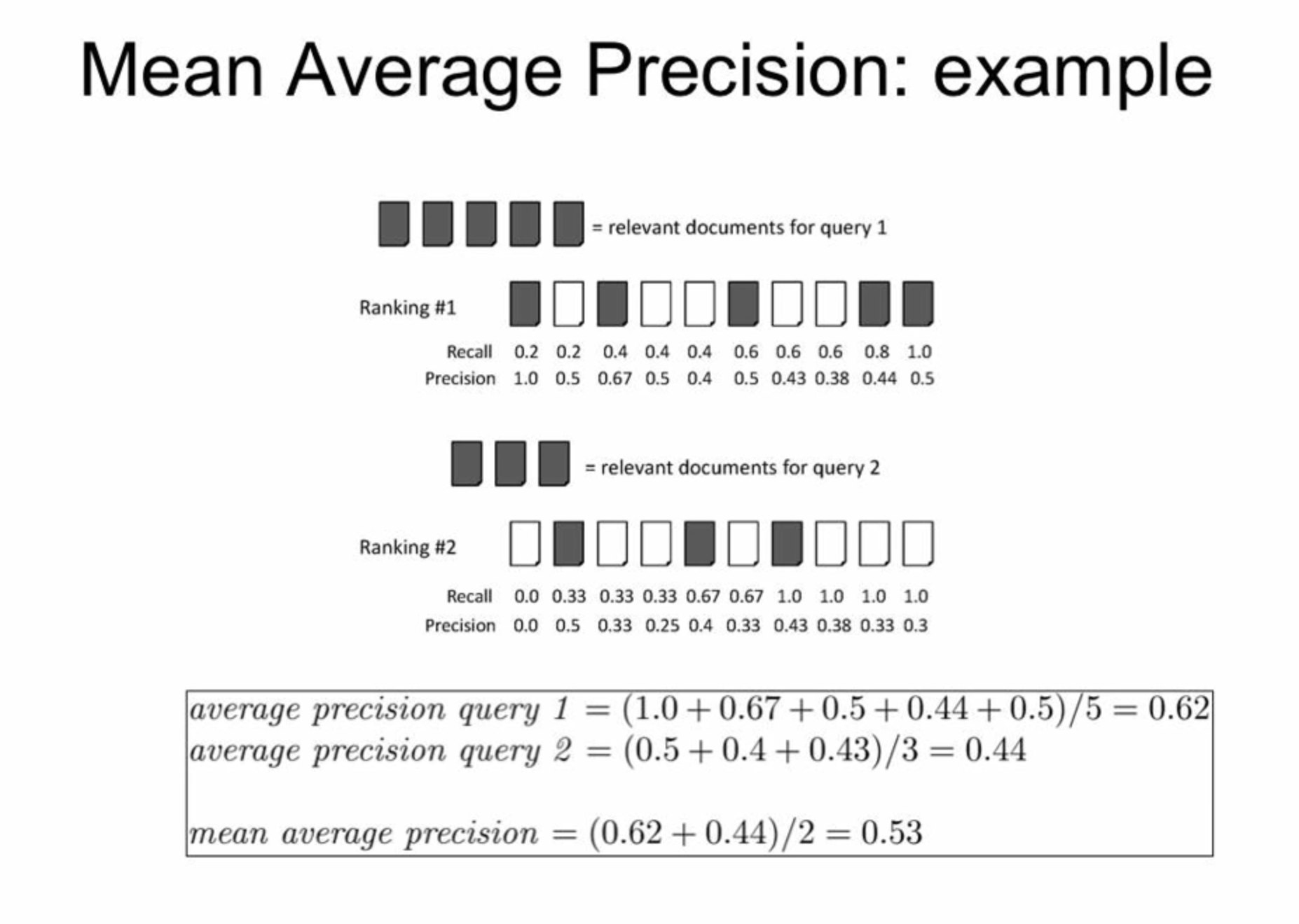
MAP extends the idea of AP to a set of queries (searches). It is the mean of the Average Precision scores for each query. Here’s how it’s generally calculated:
-
For each query:
- Compute the precision at each rank in the list of retrieved items.
- Calculate the AP by taking the average of these precision values at each rank where a relevant item is found.
-
For the dataset:
- Calculate the mean of these AP scores over all queries to get MAP.
Formula
If we have ( Q ) queries, and for each query ( q ), ( n_q ) is the number of retrieved items, and ( P(k, q) ) is the precision at cut-off ( k ) in the list for query ( q ), then MAP is calculated as:
where ( \text{rel}(k, q) ) is an indicator function equaling 1 if the item at rank ( k ) is a relevant document for query ( q ), and 0 otherwise.
MAP is particularly useful in scenarios where you want to understand how well your system retrieves all relevant documents and also how well it ranks them. It’s widely used in:
- Search engines.
- Recommender systems.
- Image retrieval systems.
- Any domain where the order of retrieval is as important as the retrieval itself.
↳ Where else would mAP be useful?
- Search engines.
- Recommender systems.
- Image retrieval systems.
- object detection (i.e. localisation and classification). Localization determines the location of an instance (e.g. bounding box coordinates) and classification tells you what it is (e.g. a dog or cat).
- Segmentation systems
- Any domain where the order of retrieval (ranking) is as important as the retrieval itself
Mean Average Precision(mAP) is a metric used to evaluate object detection models such as Fast R-CNN, YOLO, Mask R-CNN, etc.
↳ Where else would mAP be useful?
Can you write a Python function to implement m
GMAP
Geometric Means
In general, geometric means are good for !$$ \left(\prod {i=1}^{n}x{i}\right)^{\frac {1}{n}}={\sqrt[{n}]{x_{1}x_{2}\cdots x_{n}}}
\text{Cross Entropy} = -\sum_{x} T(x) \log_2 P(x)