Principal Component Analysis

Video 1: https://youtu.be/g-Hb26agBFg?si=LrdeAZu38WPH2ieY Video 2: https://youtu.be/FgakZw6K1QQ?si=SftL4BCkw8FCVKD2 https://youtu.be/oRvgq966yZg?si=my4rpbmbpYzxZMZ2 Video 3: https://youtu.be/FD4DeN81ODY?si=AA1Jc_1BXs4vTJxz Website 1: https://devopedia.org/principal-component-analysis

PCA (explanation 1)

The idea is to reduce the number of variables in a dataset while preserving as much information as possible. This is done by transforming the original variables into a new set of variables, the principal components, which are uncorrelated and ordered so that the first few retain most of the variation present in all of the original variables

PCA (explanation 2)

PCA is a statistical procedure that uses an orthogonal transformation to convert a set of observations of possibly correlated variables into a set of values of linearly uncorrelated variables called principal components.

PCA (explanation 3)

Principal Component Analysis (PCA) is a statistical technique that transforms the data into a new coordinate system, such that the greatest variance by any projection of the data comes to lie on the first coordinate (called the first principal component), the second greatest variance on the second coordinate, and so on.

PCA extracts new features which are:

1. Ranked in order of importance
2. Orthogonal to each other

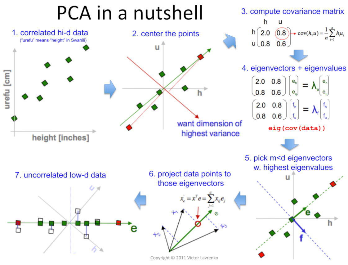
Steps:

PCA finds the best fitting line by maximising the sum of squared distances from the projected points to the origin.

Practical tips:

• Make sure your data are on the same scale (by scaling or standardising)
• Make sure your data is centered
• PC1 > PC2. The number of principal components

So theres how much variation each PC is respondible for ANd then there’s like the linear breakdown of each PC

Eigen value = the sum of squared distances

Drawbacks §

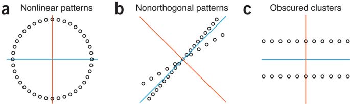
1. PCA only works with linearly correlated data. If there is correlation, PCA will fail to capture adequate variance with fewer components.
2. PCA is lossy compression
3. Scale of variables can affect results
4. Principal components are linear combinations of the original features, and can thus their meaning can be hard to interpret.

The mathematics §

☞ We are going to project each datapoint onto a line.

☞ Let’s see how we would project a single point onto a line. We will represent the line by a unit vector $\vec{u}$. You should know from vector projections that the projection of datapoint $x$, $x^{\prime }$, onto the unit vector is simply:

$$x^{\prime }=(x^{T}u)u$$

In a more familiar but equivalent form:

$$pro{j}_{u}x=\frac{x\cdot u}{||u|{|}^2}u=(x\cdot u)u$$

☞ Note that $(x^{T}u{)}^2=(x\cdot x{)}^2$ represents the information preserved after projection onto $u$.

☞ You should understand from your dot product rules that this ‘information preserved’ quantity is maximal when $x$ is parallel to $u$, and minimal when $x$ is orthogonal (perpendicular) to $u$.

☞ The optimization problem thus becomes: to find a unit vector $u$ which maximizes this information preserved quantity.

$$\text{max}\sum _i(x_i^{T}u{)}^2$$

Subject to the constraint: $u^{T}u=1$ or in other words, $u$ is a unit vector.

Note that $u$ represents the unit vector we are trying to find, and $x_1,x_2,\dots$ are the fixed observations.

☞ We use Lagrange Multiplies to solve this optimization problem. First, simplify the objective function:

$$\text{max }{u}^{T}Cu$$

Where

$$C=\frac{1}{n}\sum _i{x}_i{x}_i^T$$

is a covariance matrix representing the variance/covariance between each variable. Note that the covariance matrix calculation is simplified since the mean of the data is assumed to be zero. The full calculation to find the covariance matrix can be found here.

☞ Then form the Lagrange function:

$$\begin{array}{rl}\mathcal{L}& =u^{T}Cu-\lambda (u^{T}u-1)\\ \frac{\partial \mathcal{L}}{\partial u}& =2Cu-2\lambda u=0\\ \therefore Cu& =\lambda u\end{array}$$

Thus, we know that the direction which preserves the most information after projection is given by $u$. $u$ happens to be an eigenvalue of $C$. Interestingly, the total amount of information preserved is $\lambda$, since:

$$\begin{array}{rl}\lambda & =u^{T}Cu\\ \lambda & =\sum _i(x_i^{T}u{)}^2\end{array}$$

☞ Now, simply choose the eigenvalue with the largest eigenvector to get the first principal component. We will now look at how to get the second principal component.

☞ Ideally, the second PC is a unit vector that does not contain information that is already contained in the first component. Geometrically, this means that PC2 should be a unit vector in the subspace orthogonal to PC1. So therefore, we are just completing the same optimization problem with one additional constraint:

$$u_2\perp u_1$$

☞ The takeaway is that the principal components are exactly equal to the eigenvectors of the covariance matrix, and the eigenvalues tell you the amount of information preserved after projecting the data onto each principal component - indicating their importance.

☞ An $n\times n$ covariance matrix will have $n$ eigenvectors (principal components) that are all perpendicular to each other, along with $n$ associated eigenvalues.

☞ A final cool thing we can do is calculate the relative proportions of each eigenvalue ${\lambda }_1,{\lambda }_2,\dots ,{\lambda }_n$ in order to gain a proxy for the ‘importance’ of the corresponding eigenvectors. You do this by dividing each eigenvalue by the sum of all eigenvalues.