I include this because it is iconic, a great way to practice linear algebra, and one of many traditional solutions to recommender systems.
In 2006, Netflix announced the * Netflix Prize*, a million-dollar competition for finding an algorithm that beat Netflix' existing movie recommender systems.
I highly recommend you watch this video (shorter) or this one(longer), or this one (stanford).
Understanding the idea

user/item matrix
Dependencies: as usual in ML, we are exploiting structure, signal in data.
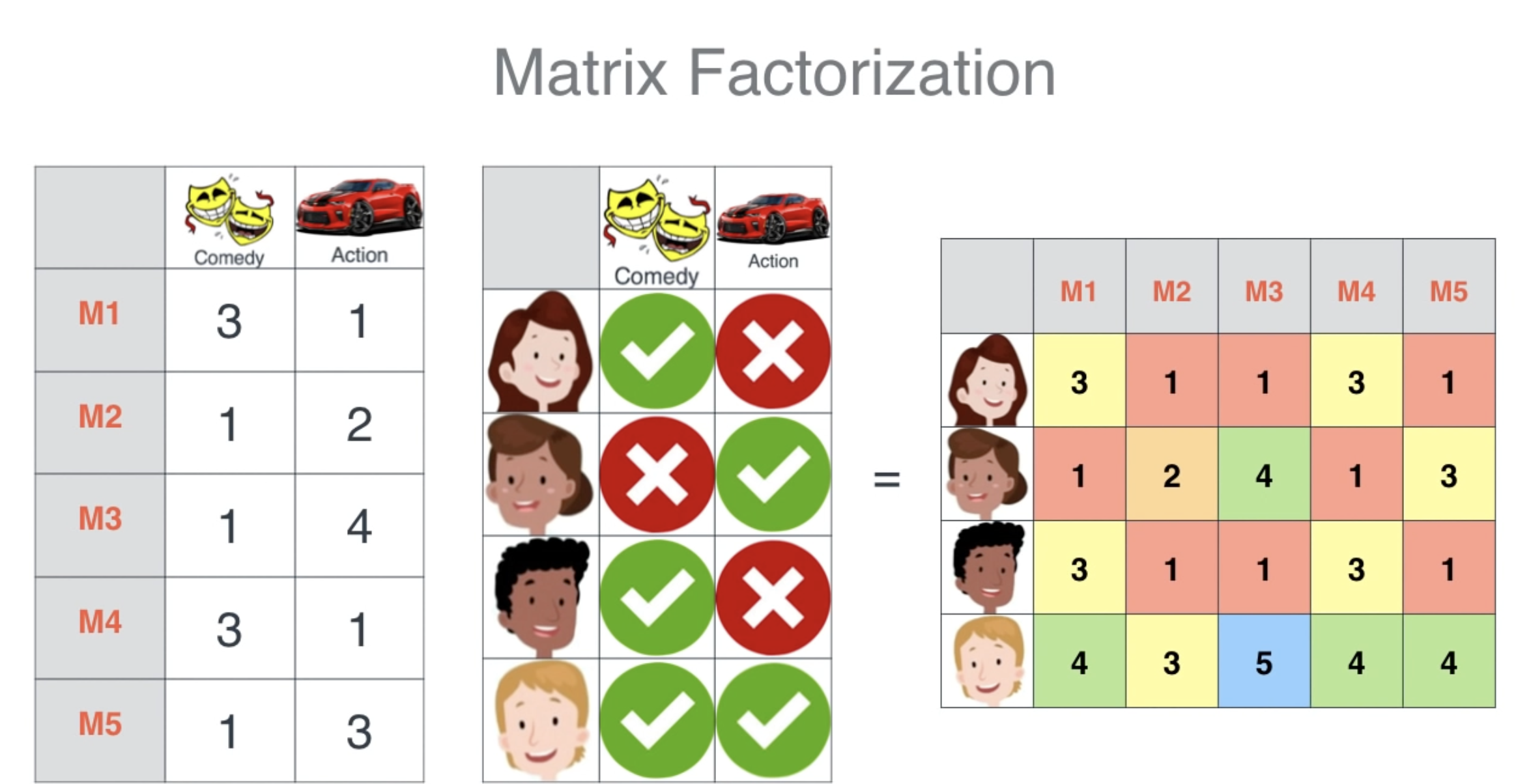
Factorization
Features:
- comedy
- drama action
- scary
- has big boat
- has sad dog
- is meryl streep in it
- does it have guy named rya
Dot product:
Storage saving for free
Collaborative filtering
The problem with user x item matrices is that they are extremely sparse, and thus lack the data to make confident predictions about a user’s preferences. One way to combat this is through simple mean imputation, as used in this question.
In 2009, a team called BellKor’s Pragmatic Chaos, found a better way, using matrix multiplication.
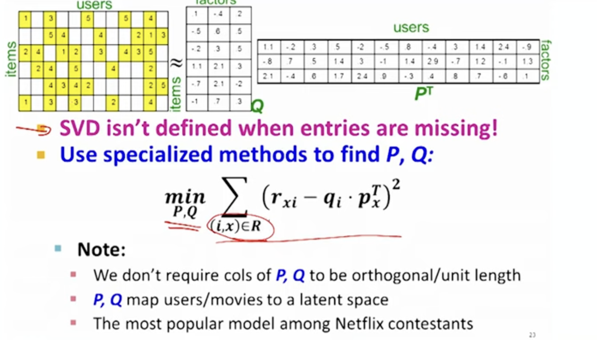
The core idea is to factorize this user-item matrix into two lower-dimensional matrices:
- A user matrix (), where each row represents a user and each column represents a latent factor.
- An item matrix (), where each row represents an item and each column represents a latent factor.
These latent factors are representative of underlying characteristics that determine how users rate items.
The Role of Matrix Multiplication:
-
Reconstructing the Original Matrix: After factorizing the original user-item matrix into the user and item matrices, matrix multiplication is used to reconstruct the original matrix. The product of the user matrix (U) and the item matrix (I) gives a new matrix that approximates the original user-item matrix.
-
Predicting Missing Ratings: The reconstructed matrix has values for all user-item pairs, including those that were missing in the original matrix. These new values are the system’s predictions for how a user would rate an item they haven’t rated yet.
Example:
Imagine a simple case with 3 users and 3 items, and the user-item matrix looks like this:
   Item1  Item2  Item3
U1   5      ?      2
U2   3      4      ?
U3   ?      1      4
After factorization and applying matrix multiplication, we get:
   Item1  Item2  Item3
U1   5     3.5    2
U2   3      4     2.5
U3   4      1     4
Here, the ”?” marks are filled with predicted ratings.
Advantages:
-
Handling Sparsity: This approach effectively deals with the sparsity of the original user-item matrix by filling in missing entries.
-
Capturing Hidden Features: The latent factors in the user and item matrices capture hidden features that might affect user preferences, such as genre in movies or author style in books.
-
Scalability: Once the factorization is done, generating predictions for any user-item pair is computationally efficient.
Conclusion:
Matrix multiplication in recommender systems provides a powerful tool for uncovering latent relationships between users and items, enabling the system to predict user preferences and make personalized recommendations. The effectiveness of these systems in capturing complex patterns and preferences hinges significantly on this mathematical operation.
Finding latent factors in recommender systems, particularly those using matrix factorization techniques, involves a process of decomposing the original user-item rating matrix into matrices representing latent factors. Let’s walk through a basic example to illustrate this process. We’ll use a simplified version of matrix factorization without regularization or bias terms for clarity.
Example Problem
Suppose we have a user-item rating matrix ( R ) with 3 users and 3 items. The ratings range from 1 to 5, and some ratings are missing (denoted by ’?’):
[ R = \begin{bmatrix} 5 & ? & 2 \ 3 & 4 & ? \ ? & 1 & 4 \end{bmatrix} ]
Our goal is to factorize ( R ) into two matrices ( U ) (user matrix) and ( I ) (item matrix), where each matrix has latent factors. Let’s say we choose to have 2 latent factors. So, ( U ) is a 3x2 matrix and ( I ) is a 2x3 matrix.
Step 1: Initialize the Matrices
We start by initializing ( U ) and ( I ) with some random values:
[ U = \begin{bmatrix} 0.1 & 0.6 \ 0.7 & 0.2 \ 0.5 & 0.3 \end{bmatrix}, \quad I = \begin{bmatrix} 0.9 & 0.4 & 0.2 \ 0.3 & 0.8 & 0.5 \end{bmatrix} ]
Step 2: Matrix Factorization
We aim to find ( U ) and ( I ) such that their product approximates ( R ) as closely as possible. This is typically done using an iterative optimization technique like Stochastic Gradient Descent (SGD). We define an error function, such as the mean squared error of the known ratings:
[ \text{Error} = \frac{1}{N} \sum (r_{ui} - \hat{r}_{ui})^2 ]
where ( r_{ui} ) is the actual rating by user ( u ) for item ( i ), ( \hat{r}_{ui} ) is the predicted rating (the product of ( U ) and ( I )), and ( N ) is the number of known ratings.
Step 3: Optimization
We then iteratively update ( U ) and ( I ) to minimize the error. In each iteration, for each known rating ( r_{ui} ), we:
-
Compute the predicted rating ( \hat{r}_{ui} = U_u \cdot I_i ) (dot product of the user’s and item’s latent factor vectors).
-
Compute the error ( e_{ui} = r_{ui} - \hat{r}_{ui} ).
-
Update the factors in ( U ) and ( I ) using the gradients of the error with respect to these factors:
[ U_u = U_u + \alpha \cdot e_{ui} \cdot I_i ] [ I_i = I_i + \alpha \cdot e_{ui} \cdot U_u ]
where ( \alpha ) is the learning rate.
This process is repeated until the error converges to a minimum or a maximum number of iterations is reached.
Example Iteration
Let’s say we compute the predicted rating for the first known rating (user 1, item 1, rating = 5):
-
( \hat{r}_{11} = [0.1, 0.6] \cdot [0.9, 0.3]^T = 0.27 )
-
( e_{11} = 5 - 0.27 = 4.73 )
-
Update ( U_1 ) and ( I_1 ) (assuming ( \alpha = 0.01 )):
[ U_1 = [0.1, 0.6] + 0.01 \cdot 4.73 \cdot [0.9, 0.3] ] [ I_1 = [0.9, 0.3] + 0.01 \cdot 4.73 \cdot [0.1, 0.6] ]
Conclusion
This example simplifies several aspects (like regularization to prevent overfitting) but captures the essence of how latent factors are found in matrix factorization for recommender systems. The process involves initializing matrices, iteratively updating them to minimize prediction error, and ultimately using the product of these matrices to predict unknown ratings.
Once the latent factors for users and items are identified through matrix factorization, reconstructing (or approximating) the original user-item matrix with imputed values for the missing ratings is a matter of performing a matrix multiplication of the user and item matrices. This step produces a fully populated matrix where each entry represents a predicted rating, including those that were originally missing.
Continuing from the previous example, let’s say we have our final user matrix ( U ) and item matrix ( I ) after the optimization process. Let’s assume these are the matrices:
[ U = \begin{bmatrix} a & b \ c & d \ e & f \end{bmatrix}, \quad I = \begin{bmatrix} w & x & y \ z & m & n \end{bmatrix} ]
The reconstructed matrix ( R’ ) is obtained by the matrix multiplication of ( U ) and ( I ):
[ R’ = U \times I ]
[ R’ = \begin{bmatrix} a & b \ c & d \ e & f \end{bmatrix} \times \begin{bmatrix} w & x & y \ z & m & n \end{bmatrix} ]
[ R’ = \begin{bmatrix} aw+bz & ax+bm & ay+bn \ cw+dz & cx+dm & cy+dn \ ew+fz & ex+fm & ey+fn \end{bmatrix} ]
Each element of ( R’ ) (say ( R’_{ij} )) represents the predicted rating of user ( i ) for item ( j ). For users and items with known ratings, these values are approximations of the original ratings. For users and items with previously unknown ratings (denoted by ’?’), these values are the new predictions filled in by the recommender system.
Example Calculation
Let’s do a sample calculation with hypothetical values for the matrices:
Assuming: [ U = \begin{bmatrix} 0.5 & 0.6 \ 0.7 & 0.2 \ 0.3 & 0.8 \end{bmatrix}, \quad I = \begin{bmatrix} 0.9 & 0.4 & 0.2 \ 0.1 & 0.7 & 0.5 \end{bmatrix} ]
The reconstructed matrix ( R’ ) is: [ R’ = \begin{bmatrix} 0.5 \times 0.9 + 0.6 \times 0.1 & 0.5 \times 0.4 + 0.6 \times 0.7 & 0.5 \times 0.2 + 0.6 \times 0.5 \ 0.7 \times 0.9 + 0.2 \times 0.1 & 0.7 \times 0.4 + 0.2 \times 0.7 & 0.7 \times 0.2 + 0.2 \times 0.5 \ 0.3 \times 0.9 + 0.8 \times 0.1 & 0.3 \times 0.4 + 0.8 \times 0.7 & 0.3 \times 0.2 + 0.8 \times 0.5 \end{bmatrix} ]
[ R’ = \begin{bmatrix} 0.51 & 0.82 & 0.53 \ 0.65 & 0.54 & 0.34 \ 0.35 & 0.76 & 0.44 \end{bmatrix} ]
In ( R’ ), each element provides a predicted rating, including those for previously unknown user-item pairs.
Conclusion
The reconstructed matrix provides a complete picture of the predicted preferences across all users and items. It’s important to note that these are approximations and the accuracy of these predictions depends on the quality of the factorization process and the underlying data.

NOT SVD BECAUSE;