2.9.2 Support Vector Machines

The radial kernel works in infinite dimensions, I know that sounds kind of crazy, but it's actually not that bad - StatQuest

The SVM is one of the most simple and elegant ways to tackle the fundamental machine learning task of classification. - StatQuest

Visually Explained | StatQuest | Intuitive ML

Can you explain what a Support Vector Machine is and how it works?

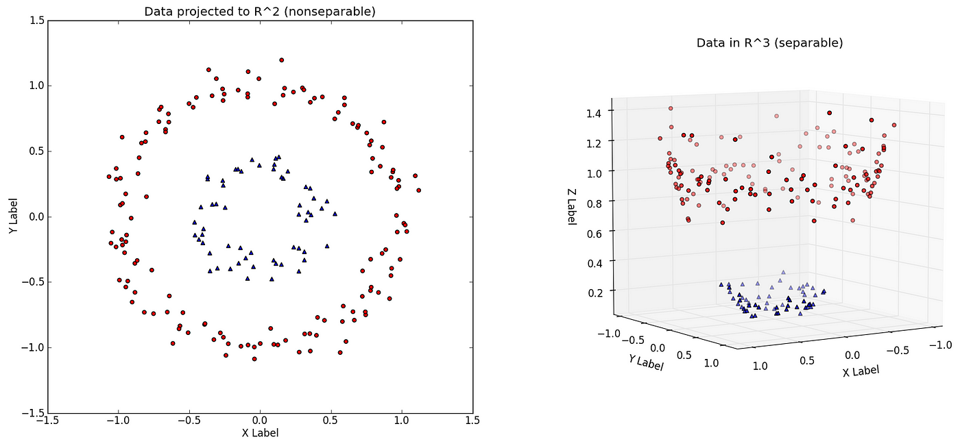
Non-Linearly Separable Data

The need for SVM’s arises when dealing with non-linearly separable data - i.e data that you cannot separate with a hyperplane (a line or plane)

A one-dimensional example:

A two-dimensional example:

So then how do SVM’s solve this? What’s the main idea?

Start with data in a relatively low dimension. Each object that we want to classify is represented as a point in an n-dimensional space.

Transform the data into a higher dimension

Find a Support Vector Classifiers that separates the higher dimensional data into two groups

Optional: project back to the original space, allowing you to see how the boundary separates the data in the original dimension. (Note: in this example the original data was 2D)

Kernel trick

A technique known as the kernel trick allows us to efficiently perform all of these steps.

↳ Is it a supervised or unsupervised machine learning model?

They are definitely supervised. The decision boundary is derived directly from the training data.

↳ Are they only useful for classification?

No! They can also be used for regression (more on this later).

When would this type of data arise (i.e data that cannot be linearly separated)’

☞ Imagine that the x-axis represents the dosage of a particular medicine. ☞ The two classes would be cured or not cured. ☞ And the yellow dots in the middle would represent the ideal dosage of medicine that should be taken to cure the patient; to little or too much is ineffective.

In the previous example, each datapoint was squared to form the new dimension. But in practice, how can you determine the best transformation?

This is true: how did we know to create a new axis consisting of $dosage^{2}$ , instead of $dosage^{3}$ , or $dosage^{0.5} + 33$ ? The answer is kernal functions

Kernel Functions

Kernel functions allow for more flexible decision boundaries by implicitly transforming data into higher dimensions.

SVM’s use kernel functions to systematically find support vector classifiers in higher dimensions.

These kernel functions transform the data in such a way that the data can then be separated by the simpler support vector classifiers using a flat hyperplane.

Note: there are many different types of kernel functions to pick from. Kernel functions are a class of functions

↳ Could you name a commonly used kernel function?

Yes, the polynomial kernel and the radial basis function.

The polynomial kernel

$K (x_{1}, x_{2}) = (x_{1} \times x_{2} + r)^{d}$

$x_{1}$ and $x_{2}$ are the two datapoints that we want to know the high-dimensional relationship between.

$r$ the polynomial’s coefficient

$d$ the degree of the polynomial And returns a number representing the high dimensional relationship between the two points.

The degree of the polynomial directly specifies the number of dimensions of the data. E.g, $d = 3$ transforms the data into $3$ dimensions $(x, y, z)$ , meaning a plane is required to separate the data into two classes.

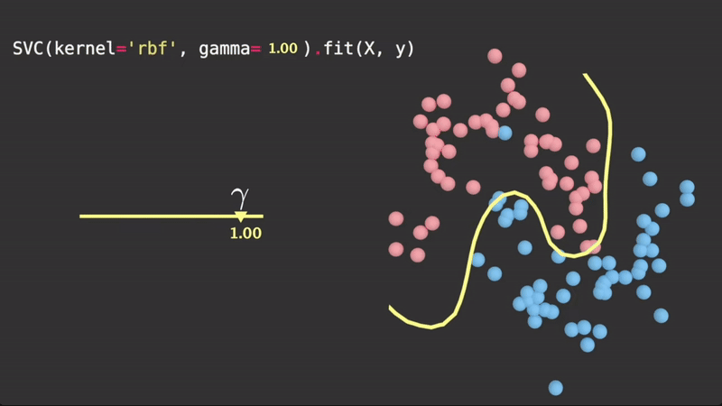
Another commonly used kernel function is called the Radial Basis Function (RBF)

Radial Basis Function

$K (x_{1}, x_{2}) = e^{- γ (x_{1} - x_{2})^{2}}$

Finds Support Vector Classifiers in infinite dimensions

Behaves like a weighted nearest neighbour model

It’s also worth mentioning the linear kernel (non-kernel).

Linear kernel

This is equivalent to using no kernel at all (also known as the non-kernel)

The linear kernel does not implicitly increase the dimensions of the data, thus the resulting hyperplane is fit in the original dimension.

The relationship between two points using the linear kernel is just their dot products with an optional constant $c$ :

$K (x_{1}, x_{2}) = x_{1} \cdot x_{2} + c$

What is the kernel trick?

Kernel trick (simple definition)

The Kernel trick is essentially what we’ve already discussed; it lets you separate data that is not linearly separable by simply adding dimensions.

Another aspect of the kernel trick is that you don’t need to actually transform all the data into the higher dimensional space, which is computationally expensive. Instead, you can simply calculate the relationships between points implicitly; as if they were in their higher-dimensional positions, without ever actually transforming the data points.

Knowing the relationships between points is all that is required in order to find the hyperplane. See the mathematics here.

Kernel trick (advanced definition)

The kernel trick is a mathematical technique used in machine learning to solve problems that are not linearly separable in their original space by implicitly mapping the input features into a higher-dimensional space. This allows the application of linear algorithms to solve non-linear problems without explicitly performing the computationally expensive transformation.

In simpler terms, imagine you have a set of points that you cannot separate with a straight line on a two-dimensional plane. The kernel trick allows you to lift these points into a higher-dimensional space (for example, by adding another dimension that you can think of as height) where you can separate them with a plane (or a hyperplane in even higher dimensions).

The beauty of the kernel trick is that you do not need to compute the coordinates of the points in this higher-dimensional space. Instead, you use a kernel function to compute the dot product (a measure of similarity) between the points as if they were in the higher-dimensional space. This dot product is all that’s needed to perform operations such as classification, regression, or clustering in the transformed space.

What type of data are SVM’s well suited for classifying?

Support Vector Machines are also good for classifying: ☞ Small datasets ☞ Data that a neural net would overfit ☞ High dimensional data ☞ Non-linear data, using Kernel Tricks

What is a binary classification task?

Read here.

Why would you use an SVM when neural networks exist?

If low amounts of high dimensional data.
If it’s data with clear segments, that neural nets are likely to overfit.
SVM’s are lightweight whereas neural networks are computationally expensive.
SVMs are simpler to implement and tune compared to neural networks, which require careful tuning of numerous hyperparameters and long training times.
Read more in this question

Anonymous Youtuber

Everyone always jumps to neural networks, but often SVMs do the same classification work with no huge iterative training required and are simply a better solution much of the time.

How do you handle imbalanced classes in logistic regression?

See the original question and answer here.

Methods specific to logistic regression:

Can SVM’s be used with categorical data, or just continuous?

Yes!

All you have to do is encode the categorical data using techniques such as one-hot encoding or binary encoding to convert the categorical variables into numerical format.

Once the categorical data has been encoded, you can then apply the SVM algorithm as you would with numerical data

What is the difference between a MMC, SVC, and a SVM? When should you use each?

☞ MMC: If the data has no outliers or noise, and is linearly separable. ☞ SVC: If the data is linearly separable. ☞ SVM: If the data is not linearly separable.

Can we talk a bit about the math behind these kernel functions? How does the polynomial kernel function allow you to calculate the high dimensional relationships between points?

We will again break the mathematics down into a sequence of logical steps. Make sure you understand the math behind support vector classifiers first.

The polynomial kernel function: $(x_{1} \times x_{2} + r)^{d}$ works like this: $x_{1}$ and $x_{2}$ are two data points that we want to know the high-dimensional relationship between. Let’s let $r = \frac{1}{2}$ and $d = 2$ . Then,

(x_{1} \times x_{2} + \frac{1}{2})^{2} = (x_{1} \times x_{2} + \frac{1}{2}) (x_{1} \times x_{2} + \frac{1}{2}) = x_{1} x_{2} + x_{1}^{2} x_{2}^{2} + \frac{1}{4} = x_{1}^{2} x_{2}^{2} + x_{1} x_{2} + \frac{1}{4} = (x_{1}, x_{1}^{2}, \frac{1}{2}) \cdot (x_{2}, x_{2}^{2}, \frac{1}{2})

Now, notice how the two vectors in the dot product represent the point vectors (coordinates) of the points in the higher dimension? Note that we can ignore the $\frac{1}{2}$ at the end, as this component of the vector will always be a double up.

(x_{1}, x_{1}^{2}, \frac{1}{2}) \to (x_{1}, x_{1}^{2})

So this is how the polynomial kernel function implicitly maps the data points to their positions in higher dimensions.

All you need to do is plug values into $x_{1}$ and $x_{2}$ in the kernel to get the high dimensional relationships between two points. Notice how if you only observe the input and output of the kernel equation, the data is never actually transformed. This, again, is the kernel trick.

Can you please go through the math for the radial basis function?

Step 1

e^{- γ (x_{1} - x_{2})^{2}} = the high-dimensional relationship

The radial kernel (radial basis function (RBF)) determines how much influence each observation has on classifying new observations.

For any two observations $x_{1}$ and $x_{2}$ , we get the squared distance between them with $(x_{1} - x_{2})^{2}$

$γ$ is a scalar parameter which scales this squared distance, and thus scales the influence. Geometrically, it controls how tightly the hyperplane fits the data. It is determined via cross validation. A visualization of $γ$ :

Taken from Visually Explained

Since this squared distance function is part of an $e^{- x}$ function, clearly the larger the squared distance between two observations, the lower the value of the $RBF$ , due to the decaying nature of $e^{- x}$ .

Step 2

Now, we must take a step back and consider a polynomial kernel function again. If we let the coefficient $r = 0$ , the function simplifies to:

(x_{1} \times x_{2} + r)^{d} = (x_{1} \times x_{2})^{d} = (x_{1}^{d} \cdot x_{2}^{d}) = (x_{1}^{d}) \cdot (x_{2}^{d})

Notice how the vectors in the resulting dot product only have one component. Thus, when $r = 0$ , all the polynomial kernel does is shift the data down its original axis, by raising it to the power $d$ .

I.e $x_{1} \to x_{1}^{2}$

So setting $r$ to $0$ seems pointless, since the dot products leave the data in their original dimension.

Step 3

If we add the $r = 0, d = 1$ case to the $r = 0, d = 2$ case, the result becomes:

x_{1} x_{2} + x_{1}^{2} x_{2}^{2} = (x_{1}, x_{1}^{2}) \cdot (x_{2}, x_{2}^{2})

If we let $d \to \infty$

x_{1} x_{2} + x_{1}^{2} x_{2}^{2} + x_{1}^{3} x_{2}^{3} + \dots = (x_{1}, x_{1}^{2}, x_{1}^{3}, \dots) \cdot (x_{2}, x_{2}^{2}, x_{2}^{3}, \dots)

Notice how we can convert this series into a dot product.

Step 4

Now, let’s revisit the original radial basis function and expand the quadratic in the power.

e^{- γ (x_{1} - x_{2})^{2}} = e^{- γ (x_{1}^{2} + x_{2}^{2} - 2 x_{1} x_{2})} = e^{- γ (x_{1}^{2} + x_{2}^{2})} e^{γ 2 x_{1} x_{2}}

Letting $γ = \frac{1}{2}$ to simplify the $2 ab$

= e^{- \frac{1}{2} (x_{1}^{2} + x_{2}^{2})} e^{x_{1} x_{2}}

Step 5

Now let’s find the Taylor Series Expansion of the last term, $e^{x_{1} x_{2}}$ . We know that the central ( $a = 0$ ) Taylor series expansion of $e^{x}$ is:

e^{x} = 1 + \frac{1}{1 !} x + \frac{1}{2 !} x^{2} + \frac{1}{3 !} x^{3} + \dots + \frac{1}{\infty !} x^{\infty}

Now simply let $x = x_{1} x_{2}$ to get

e^{x_{1} x_{2}} = 1 + \frac{1}{1 !} x_{1} x_{2} + \frac{1}{2 !} (x_{1} x_{2})^{2} + \frac{1}{3 !} (x_{1} x_{2})^{3} + \dots + \frac{1}{\infty !} (x_{1} x_{2})^{\infty}

Step 6

Notice that each term in this Taylor Series Expansion contains a polynomial kernel with $r = 0$ and $d = 0, 1, \dots, \infty$

Again, we can change the series into a dot product, but this time with square rooted coefficients so that it all works out.

e^{x_{1} x_{2}} = (1, \frac{1}{1 !} x_{1}, \frac{1}{2 !} x_{1}^{2}, \frac{1}{3 !} x_{1}^{3}, \dots, \frac{1}{\infty !} x_{1}^{\infty}) \cdot (1, \frac{1}{1 !} x_{2}, \frac{1}{2 !} x_{2}^{2}, \frac{1}{3 !} x_{2}^{3}, \dots, \frac{1}{\infty !} x_{2}^{\infty})

Step 7

Now, substitute this $e^{x_{1} x_{2}}$ back into the original radial basis function, and let $b = e^{- \frac{1}{2} (x_{1}^{2} + x_{2}^{2})}$ for simplicity. Then:

e^{- \frac{1}{2} (x_{1} - x_{2})^{2}} = (s, s \frac{1}{1 !} x_{1}, s \frac{1}{2 !} x_{1}^{2}, \dots, s \frac{1}{\infty !} x_{1}^{\infty}) \cdot (s, s \frac{1}{1 !} x_{2}, s \frac{1}{2 !} x_{2}^{2}, \dots, s \frac{1}{\infty !} x_{2}^{\infty})

Finally, we see that the radial kernel for points $x_{1}$ and $x_{2}$ is equal to the dot product of two vectors with an infinite number of dimensions.

For example, take the datapoints 2 and 3. Simply computing

e^{- \frac{1}{2} (2 - 3)^{2}} = 0.6065

gives us their infinite-dimensional relationship, encapsulated within a single value.

Now that you’ve used the kernel trick to calculate high-dimensional relationships between points, how can you use this to actually find the hyperplane mathematically?

How would you go about implementing a SVM on a dataset about (), using `Python`? You have the following data:

# observations (a list of feature vectors)
X = [ [-3, -1], 
	  [0, -2], 
	  [-2.5, 2], 
	  [-1, -1], 
	  [3, .5], 
	  [.5, 3], 
	  [-3, -3] ] 
 
# classifications 
y = [0, 1, 0, 1, 1, 0, 1]

Training and using a SVM can literally be done in 4 lines of code:

from sklearn import svm
clf = svm.SVC(kernel = 'linear')
clf.fit(X, y)
clf.predict([[2, 4], [3, 3.5]])

The output:

[0, 1]

Meaning the first datapoint belongs to class 0, and the other one belongs to class 1

⚘ DSX.com

Explorer

2.9.2 Support Vector Machines

Can you explain what a Support Vector Machine is and how it works?

So then how do SVM’s solve this? What’s the main idea?

↳ Is it a supervised or unsupervised machine learning model?

↳ Are they only useful for classification?

When would this type of data arise (i.e data that cannot be linearly separated)’

In the previous example, each datapoint was squared to form the new dimension. But in practice, how can you determine the best transformation?

↳ Could you name a commonly used kernel function?

What is the kernel trick?

What type of data are SVM’s well suited for classifying?

What is a binary classification task?

Why would you use an SVM when neural networks exist?

How do you handle imbalanced classes in logistic regression?

Methods specific to logistic regression:

Can SVM’s be used with categorical data, or just continuous?

What is the difference between a MMC, SVC, and a SVM? When should you use each?

Can we talk a bit about the math behind these kernel functions? How does the polynomial kernel function allow you to calculate the high dimensional relationships between points?

Can you please go through the math for the radial basis function?

Step 1

Step 2

Step 3

Step 4

Step 5

Step 6

Step 7

Now that you’ve used the kernel trick to calculate high-dimensional relationships between points, how can you use this to actually find the hyperplane mathematically?

How would you go about implementing a SVM on a dataset about (), using `Python`? You have the following data:

Graph View

Backlinks

⚘ DSX.com

Explorer

2.9.2 Support Vector Machines

Can you explain what a Support Vector Machine is and how it works? §

So then how do SVM’s solve this? What’s the main idea? §

↳ Is it a supervised or unsupervised machine learning model? §

↳ Are they only useful for classification? §

When would this type of data arise (i.e data that cannot be linearly separated)’ §

In the previous example, each datapoint was squared to form the new dimension. But in practice, how can you determine the best transformation? §

↳ Could you name a commonly used kernel function? §

What is the kernel trick? §

What type of data are SVM’s well suited for classifying? §

What is a binary classification task? §

Why would you use an SVM when neural networks exist? §

How do you handle imbalanced classes in logistic regression? §

Methods specific to logistic regression: §

Can SVM’s be used with categorical data, or just continuous? §

What is the difference between a MMC, SVC, and a SVM? When should you use each? §

Can we talk a bit about the math behind these kernel functions? How does the polynomial kernel function allow you to calculate the high dimensional relationships between points? §

Can you please go through the math for the radial basis function? §

Step 1 §

Step 2 §

Step 3 §

Step 4 §

Step 5 §

Step 6 §

Step 7 §

Now that you’ve used the kernel trick to calculate high-dimensional relationships between points, how can you use this to actually find the hyperplane mathematically? §

How would you go about implementing a SVM on a dataset about (), using Python? You have the following data: §

Graph View

Backlinks

Can you explain what a Support Vector Machine is and how it works?

So then how do SVM’s solve this? What’s the main idea?

↳ Is it a supervised or unsupervised machine learning model?

↳ Are they only useful for classification?

When would this type of data arise (i.e data that cannot be linearly separated)’

In the previous example, each datapoint was squared to form the new dimension. But in practice, how can you determine the best transformation?

↳ Could you name a commonly used kernel function?

What is the kernel trick?

What type of data are SVM’s well suited for classifying?

What is a binary classification task?

Why would you use an SVM when neural networks exist?

How do you handle imbalanced classes in logistic regression?

Methods specific to logistic regression:

Can SVM’s be used with categorical data, or just continuous?

What is the difference between a MMC, SVC, and a SVM? When should you use each?

Can we talk a bit about the math behind these kernel functions? How does the polynomial kernel function allow you to calculate the high dimensional relationships between points?

Can you please go through the math for the radial basis function?

Step 1

Step 2

Step 3

Step 4

Step 5

Step 6

Step 7

Now that you’ve used the kernel trick to calculate high-dimensional relationships between points, how can you use this to actually find the hyperplane mathematically?

How would you go about implementing a SVM on a dataset about (), using `Python`? You have the following data: